


Some things just aren’t fair. With no spending floors or ceilings in Major League Baseball, a given team can spend whatever they like in a given year. It is not uncommon to see one team spend 5x more than a smaller-market counterpart, with both expected to compete equally. For the sake of hypotheticals, let’s imagine a scenario where baseball spending is completely fair. All teams spend the same amount – there is total equality in cash spent numbers. Teams can no longer rely on their insane spending power to grant that edge, completely changing the game. Which teams would thrive? Which teams would fail? Answering these questions and more with 100% certainty is not possible, but there can be a well-thought-out projection. For this piece, that projection will be called CAW%, or Cash-Adjusted Win Percentage.
Methodology
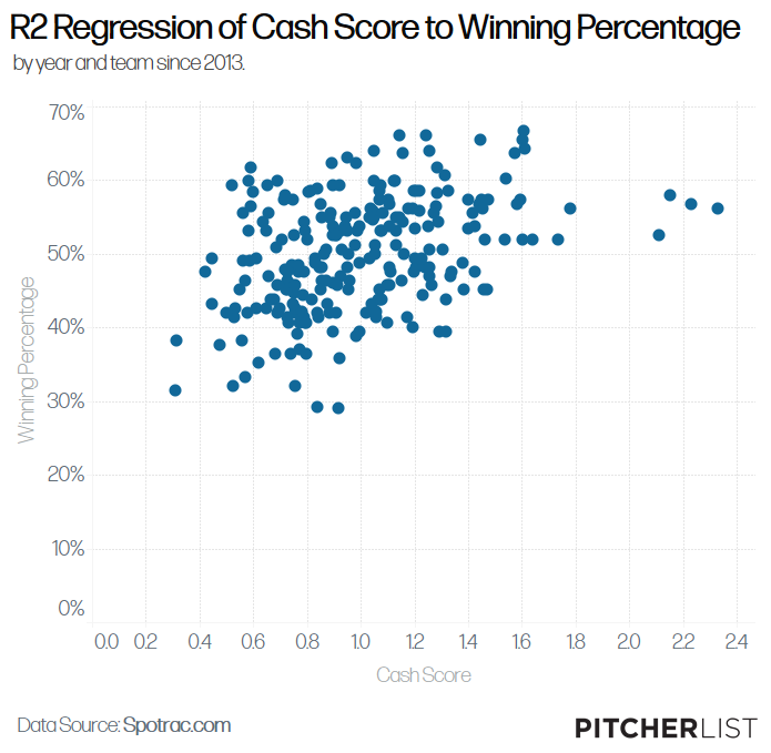
While the projection has the word cash in it, the entire point of this exercise was to completely isolate the cash variable from the equation. After all, in a perfectly equal spending environment, cash does not matter. To successfully isolate that variable, the effect that cash had on winning needed to be articulated. I mentioned earlier that there is an effect, but without knowing the extent of that effect, this measurement would be useless. To solve this, I conducted a basic linear regression. Using win percentages for each team and total cash spending data (which was adjusted for MLB spending inflation) from 2013-2021 (excluding 2020), this regression was able to show an r-squared score between the two aforementioned variables. During the sample used, total adjusted cash spent accounted for 15.8% of win percentages – spending money provided a serious boost. The actual regression is shown here:
Created by @visual_endgame on Instagram & Twitter.
Of course, the actual r-squared for cash spent does vary based on what samples are being used (generally accounting for 10-20% of Win Percentage from prior personal research). For this study, 15.8% was utilized as it is the most accurate for this specific sample. In a possible reproduction of this, the percentage should be based on the given r-squared between the two factors within the sample. This percentage was used to split between two variables – cash-dependent winning percentage and non-dependent cash winning percentage. Cash-dependent winning percentage takes 15.8% of the total winning percentage (the amount that was dependent on cash) of a given team and weighs it based on a given team’s total cash spent. Non-dependent cash winning percentage is just the percentage left over; it is the 84.2% that cash spending did not impact. The separation of these two factors laid the framework for the actual formula.
The only factor that needed to be adjusted is the cash-dependent winning percentage variable. The non-dependent version was left in its nominal form, as it has nothing to do with cash – other irrelevant factors likely impacted it. It was mentioned that the cash-dependent version would be weighted based on total cash spent, but it is not as simple as just taking the total dollar amount used. The amount of spending varies by year, with a general upwards trend being demonstrated. Therefore, everything needed to be made relative to the given year. This was done using cash scores, which took the amount of total cash spent by a team and divided it by the MLB average of that year. A score of 1 was to be considered average, while anything above is a percentage more and anything below is a percentage less the MLB average that year. As cash spending was properly scaled, all of the factors were to craft the equation.
Managing the weights between the two main variables and factoring them into the calculation, the formula was made as follows:
CAW% = ( (.1577814 * WP%) / Cash Score) + (.8422186 * WP%)
As mentioned, a recreation needs to adjust based on the r-squared score of the given sample between winning percentage and total cash spent, with the first weight as the r-squared score and the second weight as 1 minus the r-squared score. Other than that, the equation should work in most other scenarios pertaining to the question of an equal cash-spending baseball world.
Potential Shortcomings
Decreasing Marginal Utility of the Dollar
If you’re familiar with basic economics, you would be aware that every dollar spent does not equal one another. In the study, part of this issue was solved – but not completely. For this equation, it was assumed that dollar growth follows a linear path. If a team spends X more dollars, they will be Y better. In the real world, this is not always the case. Say the Tampa Bay Rays are put into an equal spending environment. It is known throughout baseball how smart they are and their dedication to analytics, so it is known that they would do better with more money. But as they spend more money, the value they are actually capable of adding to their already advanced infrastructure may not be equivalent to the pace that they were able to do in the past. Instead of their growth following a straight linear line, the tail-end might begin to become flat, leading to stagnation. This is not necessarily the outcome, but a regular linear line being the true outcome is also not likely. The projection should serve as a baseline for what might happen, as figuring out the possible decreased marginal utility in a more advanced projection is unlikely with public data.
Lack of Varying R-Squared Weights
Throughout the entire calculation, the r-squared weight was held constant for each season – 0.158. But, I would be askew if I did not mention that cash likely does not have the same effect every year. Using r-squared scores for each season was considered, but ultimately considered flawed. A sample of only 30 teams is too small to lead to a semi-accurate score, making it seem safer to just use the score for the entire sample and weight accordingly. In a perfect world, the sample for each season would be large enough to adjust by season. It is not a perfect world, and the calculation was adjusted accordingly.
This shortcoming will remain common in most of my pieces until I am completely satisfied with the amount of data I was able to access. Not having access to 100% accurate tracked total cash spending before the 2013 season, the study was forced to be limited to only 240 seasons. This was sizeable enough to make some conclusions, but the confidence in said conclusions would only go upward if the sample size was larger. The sample size is a crucial component in looking at all types of sabermetric data (as well as science in general), and the possible lack of a sufficient one needs to be specified in any sort of work. The reader should utilize their opinion on the sample size to take the following results with as much importance as they care to give.
The Results
After looking at what the equation yielded, the results were somewhat to be expected – they were very dependent on cash scores. The difference between a team’s CAW% and WP% with a team’s cash score had an r-squared measure of 0.834. In other words, cash scores had a very large effect on how much better or worse a team did in this adjusted measure. The results were not completely dependent on cash scores as the given success or failure in a team’s winning percentage had a sort of multiplier effect, meaning that the bigger the original winning percentage the larger the result could vary.
With the equation complete and utilized, the following are the best and worst CAW% within the sample.:
Unsurprisingly, the Rays reign supreme on these charts. They also scored similarly well during these seasons in my look at cash efficiency spending, which makes sense as they have an innate ability to produce wins for cheap. If the field was evened for cash as in this hypothetical projection, they would benefit. Oakland, San Fran, and Cleveland also made the top five, as they are notable winners that don’t spend a lot. Although not expected, the bottom five teams all spent below the average for their given seasons, having cash scores below 1. Their records were just so incredibly horrendous that even adjusting for the cash factor, they were still bad. While mathematically proven, these teams serve as clear examples that cash is not everything.
Looking at the best and the worst provides one perspective, but the general changes also needed to be reviewed. These teams exhibited the biggest absolute nominal changes between CAW% and actual winning percentage.
The range of changed winning percentages varied from losing 0.051 win percentage points (~8 losses) to adding 0.133 win percentage points (~22 wins). The former was the 2015 Los Angeles Dodgers, who went from a .562 WP% to a .511 CAW%. They were one of the biggest spenders of that year, spending 2.2 times the average MLB cash spent. In an equal spending environment, they only stood to lose. Although an incredibly articulate team, a lack of cash-spending ability would likely put them behind their lesser-spending counterparts. The latter was the 2013 Miami Marlins, who went from a .383 WP% to a .516 CAW%. Having one of the lowest cash scores in the entire sample at 0.31, an all-equal cash spending world would’ve made them an actual contender instead of a horrendous squad. The Marlins have routinely had to work with less cash due to their market size, and this seemingly has had an impact on all of their seasons during this timespan. While these are extremes at both ends, a team with a lower-than-average cash score and a somewhat excusable record (~.430 or above) had the optimized approach to benefit the most from the CAW% projection. These two factors when satisfying those criteria served as the perfect balance for success in this alternative scenario.
Conclusion
For this hypothetical world, each team was given the same means. Every team spent the same amount, with only a team’s market-savvy and innate ability to produce something from less providing them an edge. In a sense, it projects a meritocracy. With the current effects and differences between total cash spending, Major League Baseball cannot be considered a meritocracy. I intend not to muddy up the article with personal opinions regarding the notion of whether the sport should or should not change to that format – that is left up to the discretion of the reader.
When CAW% was utilized, the biggest winners were the teams that spent the least and won the most. In an all-equal world, one would have to assume that the teams that succeed now despite being at a disadvantage would only grow with more resources. The exact extent of this growth can be projected, but the variance is always possible (at least solely regarding the cash factor). The biggest losers were the opposite, although the extremes didn’t need to spend a lot to score horribly in the projection. The Baltimore Orioles spent roughly half of the average total cash spent in 2021, and still had the fifth-worst CAW%. Cash does affect records, but it is only a fraction.
Fractions may seem slight, but they govern the ultimate outcomes of the game. Fractions of cash do have a minimal effect, but often minimal effects act as dominoes that trigger big effects. They can give a few decimals to one side or another, granting one team the chance to compete in the Postseason and sending the other home. That team that was granted a chance may go on to Win, defying the ultimate odds. This is in no way inferring that money is all that matters, but it does affect the outcomes (like lots of other variable factors). The projection gave teams entirely new outlooks and chances on old seasons – who would’ve actually won the World Series? The answer to this question can never be certain, but it is clear that the entire playoff picture would’ve looked a lot different.
While CAW% was primarily presented as a hypothetical projection, it could be used for some practical applications. Specifically, what would the baseline of improved performance be for teams with more cash? It could be used to give owners a clear projection of how much they would likely improve if they spent more money, providing reasoning for them to shell out more funds. The calculation could be factored into overall team projections, with the models adjusting for the prior cash impacts and adjusting to change projected win percentages based on new cash spending. And given the right brain trust, this could have lots of other projected applications. Hypotheticals can be used as baselines, and baselines provide paths to success. The baseline that is CAW% can hopefully fulfill that very path for any team willing to consider.
Illustration by Cody Rogers (@CodyRogers10)