


Recently, I introduced Forecasted Run Average (FRA), an ERA estimator based on a combination of K-BB%, average exit velocity (aEV), and average launch angle (aLA). I billed it as more predictive of next-season ERA (S2ERA) and stickier than other publicly accessible ERA estimators: SIERA, xFIP, FIP, DRA, and xERA. True to form, I ran with FRA and tweeted it out.
However, as an attorney, statistics are not my natural domain. I haven’t taken a class on the subject in eight years. I’ve spent much of the spring learning how to program in R, and the remainder learning more about statistics. This latter effort has led me to realize that I made mistakes in developing the original FRA model and reporting its scores, necessitating this post. I want to thank Eric Colburn for acting as a sounding board in this regard.
With that said, the new model detailed below is still more predictive of future ERA than other publicly accessible ERA estimators, and is even stickier than the old model. There are a lot of great fantasy analysts coming out with new statistics every day. I want to give you a reason to trust mine.
Methods
The data sample has remained the same–all pitchers with 100 IP in back-to-back seasons since 2015 (n=352). I downloaded a wide array of over 50 variables to test from those pitchers, including, for example, xwOBAcon, ground ball rate, barrel rate, fastball%, etc. The idea was to test them against pitchers’ ERAs in the following season (S2ERA) and identify those that were most predictive. With such a large amount of predictors, I tried something different from last time. Rather than manually identifying and removing those variables presenting collinearity or those that did not improve the model, I let R do that for me.
This time, I utilized an elastic net regression to winnow down those 50 or so variables for the model. Elastic net is still a generalized linear regression, but is also a method of penalized regression that considers all variables. It just reduces the coefficient to 0 for those terms that do not improve the model, and shrinks the coefficients of those that marginally improve the model. Of course, a coefficient of 0 means that the predictor is not a part of the model, and a shrunk coefficient reduces the impact of the term.
Running the elastic net regression returned an optimal model with a high alpha (i.e., only a few predictors): K-BB%, age, aEV, FB%, average fastball speed, and zone whiff%. The model score was a 0.847 RMSE and 0.219 R2. Notably, the elastic net regression did not return aLA, so I already knew I had made a mistake in the last go around.
Three of the above variables had extremely small coefficients: FB%, average fastball speed, and zone whiff%. As a result, I decided to take an occam’s razor approach and eliminate them altogether. That, alone, as well as running a linear regression on just the three remaining variables (K-BB%, aEV, and age), improved the model’s performance (more on that later). I’ll add that the regression worked, in part, as these three have little collinearity–the strongest relationship was between K-BB% & aEV (R = -0.219).
Still, K-BB%, aEV, and age presented a different issue, as they were not all linear with S2ERA. I was able to use backward compatibility to auto-generate a line of best fit, and see whether each of the three remaining variables shared a linear relationship with S2ERA.
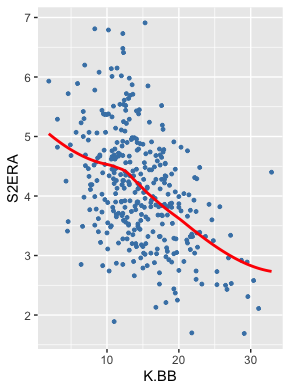
K-BB% and S2ERA do, in fact, have primarily a linear relationship. As K-BB% increases, S2ERA decreases at a similar rate. However, the same cannot be said for aEV or age. Let’s begin with the former.
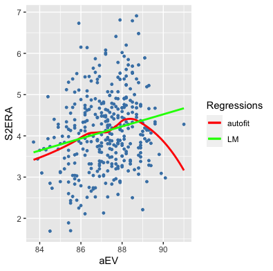
Here, I’ve plotted aEV against S2ERA, showing the auto-generated line of best fit (red) and a linear fit (green). The linear model does not best approximate the relationship between the variables, which is shown by the red line, because the green line is skewed by the high aEV data points. Using the green line would overestimate S2ERA for pitchers’ with aEVs between 83 and 86 mph, and underestimate S2ERA for those with aEVs between 86 and 89 mph.
My first thought was to use a polynomial term to capture the relationship. Yet, as I considered it further, I could find no good reason why pitchers should be rewarded in a subsequent season for a high average exit velocity in the prior season. The red line (curve?) of best fit, at the tail, actually drops below the lowest point in the beginning. Said another way, adding a polynomial term into the model to fit this curve would give pitchers with an aEV over 90 a lower S2ERA than pitchers with an aEV under 84 mph.
I think it more likely that, in general, having a high aEV is a bad omen, and this graph is just skewed by a small sample of pitchers with extremely high aEVs whose ERAs happened to drop the following year. We can tell whether a high aEV is good for ERA by plotting that relationship.
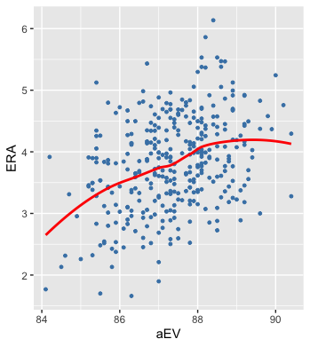
And, indeed, same-season ERA shares a more linear–albeit not perfectly linear–relationship with aEV, which means that, as we would expect, when a pitcher gets hit harder, his ERA rises, and vise versa. As noted above, however, if I just used the linear relationship between aEV and S2ERA for the model (i.e., the green line from the first plot), I would get inaccurate S2ERA predictions because the tail of the data would skew the coefficient for all pitchers’ aEVs.
To fix this and smooth out the red line from the first plot, I altered the aEVs on the tail. I changed all values of aEV above 88.3 mph to 88.3 mph as such:
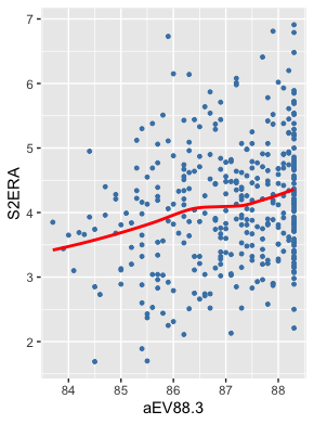
That is far more linear. The logic behind this is that, in general, we should predict a higher S2ERA if a pitcher was hit harder the year prior. We wouldn’t expect a lower ERA (as indicated by the red line on the first graph). But, both graphs also indicate there should be a limit on how high aEV can raise S2ERA. Both the S2ERA~aEV plot and the ERA~aEV plot showed diminishing returns in terms of S2ERA past around 88.3 mph. In other words, while we would expect a pitcher’s S2ERA and ERA to increase as his aEV increases, the exit velocity of balls in play only account for so much damage, thereby increasing S2ERA and ERA only until aEV reaches about 88.3 mph and then plateauing.
To that point, you can see the extreme S2ERA variability in the points at the very end of the graph, which illustrates that simply increasing (or, in the case of the red curve from the first plot, decreasing) the line at the end would not fairly capture the impact of high aEVs on S2ERA. As a compromise, I am assuming that having such a high aEV is inauspicious for future performance, but only to a point, and accordingly making the worst aEV mark 88.3 mph. I call this variable simply aEV88.3.
As an aside, many pointed out after the original FRA article that two pitchers could have the same average exit velocity while arriving at those averages in vastly different ways. It was suggested, then, to use pitchers’ xwOBAcons instead of aEVs, which grade each ball in play by the run expectancy of its launch angle and exit velocity combination. In response, I note that the elastic net regression reduced the xwOBAcon coefficient to 0. Out of an abundance of caution–and, because I understand the logic behind replacing aEV with xwOBAcon–at the end of my process I also included xwOBAcon in an Analysis of Variance (ANOVA) test. The ANOVA suggested using a model that does not include xwOBAcon, so I kept aEV88.3.
Moving on, I next visualized the relationship between age and S2ERA:
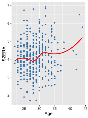
Of course, this is not linear, but it would also be difficult to find even a polynomial term to capture that relationship. Yet, I’m not surprised the elastic net regression selected age as a predictor of S2ERA, as I think there’s a clear relationship here and the curve makes sense: S2ERA rises until age 25 on the graph (i.e., through age-26 season) and then falls until age 28 (through age-29 season). Meaning that performance peaks and ERA bottoms out between ages 26-29, which makes sense to me. Then, ERA rises until age 32 on the graph (age-33 season), followed by a slight decrease and plateau. Observe also that the increase at the tail is skewed by two extremely high data points and a small sample over age 35.
Because there is a meaningful relationship here that does not present linearly, forcing a linear regression on the data as is would inaccurately capture that relationship. Doing so would simply say that, as age increases, so too does ERA the following year, which is decidedly not the case. It is clear, for example, that age 28 portends a lower S2ERA than age 25.
Accordingly, I simply reordered the ages from best to worst in terms of S2ERA by placing them in buckets in order to create a linear relationship. I scored each age by its associated S2ERA, with a higher score where an age yielded a lower S2ERA, and I attempted to maintain a normal distribution in doing so:
| Age | n | Score |
|---|---|---|
| 28 | 36 | 11 |
| 27 | 34 | 10 |
| 26 | 37 | 9 |
| 23 & 24 | 39 | 8 |
| 25 | 28 | 7 |
| 29 | 36 | 6 |
| 30 | 36 | 5 |
| 33 & 34 | 33 | 4 |
| 35+ | 24 | 3 |
| 31 | 25 | 2 |
| 22 & 32 | 24 | 1 |
And, in turn, plotting that distribution against S2ERA yields:
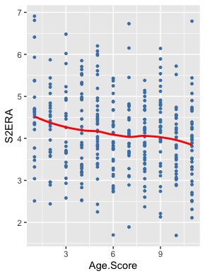
That’s much better and didn’t require altering a single data point. Significantly, as you’ll later see, substituting age scores for age and smoothing out aEV improved the model scores.
But, let me pause here to explain what I mean by “model scores.” With linear regressions, I found the coefficient of determination (R2) between the independent variables (K-BB%, aEV88.3, age score) and the dependent variable (S2ERA), which illustrates how much variance in the sample of S2ERAs is explained by the independent variables. The higher the R2, the greater the independent variables explain changes in the dependent variable (though R2 will never exceed 1).
I further found the Root Mean Squared Error (RMSE) of the model. The value of RMSE is twofold. First, it is scaled to the units of the dependent variable, so you can understand it in terms of ERA. Second, it is a measure of how spread out your model’s values are from the line of best fit. In other words, it is representative of the average error of the model’s predictions. In this case, the lower the RMSE, the lower the average error of the FRA values relative to the observed S2ERAs. RMSE is the most important measure where the main purpose of a model is prediction.
In the original FRA post, I reported that, as compared to S2ERA, FRA had an RMSE of 0.823 and an R2 of 0.245. Although I did manually split the entire dataset into training and testing sets and then test the model on the testing sets, I was reporting the scores of the model on the entire dataset, which is improper. I suspect many other fantasy baseball analysts inadvertently do something similar when they generate their own models by only running the model on the entire dataset and reporting those scores, thereby overfitting the model to the data, rather than splitting the data and running the model on data it hasn’t seen before. I myself am guilty of this, as I plainly should have used the test scores to compare FRA to other ERA estimators like SIERA and xFIP.
This time, I will not only report the test scores, but I also employed a superior method of model testing to manually splitting the data: k-fold cross-validation. The concept behind this method of testing is simple. Essentially, cross-validation iteratively splits the data set into test and training sets based on the number of k folds selected. So, if k were 5, then you’re splitting the dataset into five pieces, training the model on the first four and testing it on the fifth, then rotating the folds and repeating that process four times and, finally, averaging those five test results. We can visualize this process as such:
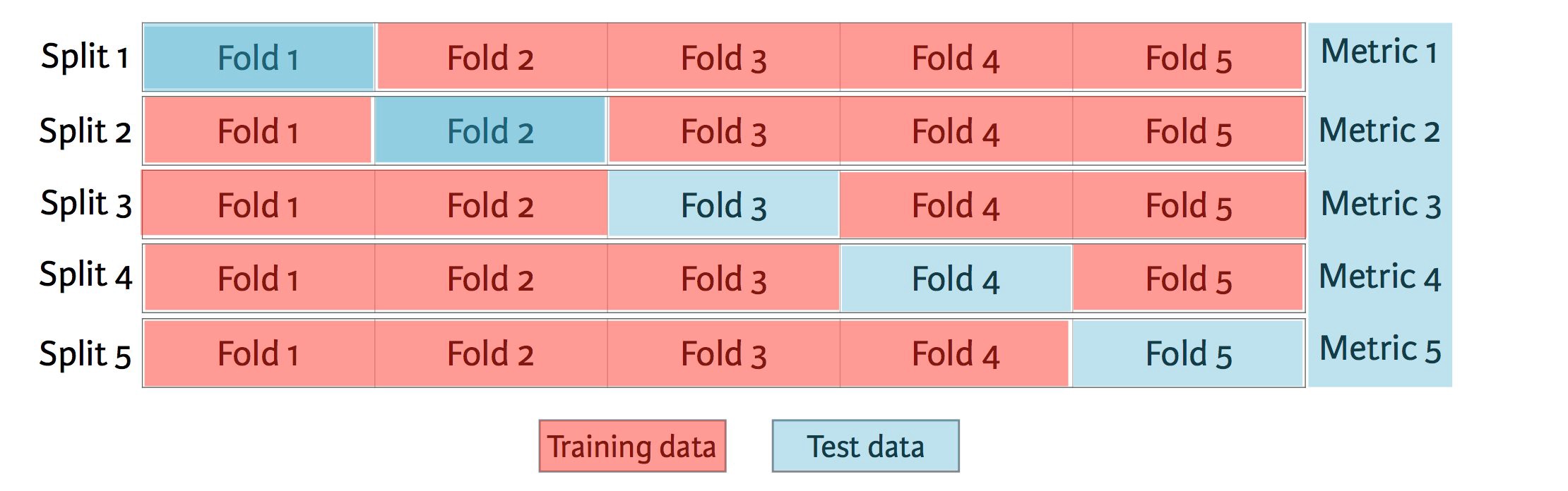
These results are then reported in terms of the average scores–RMSE and R2 in our case–across the five test folds. However, they are also reported in terms of their standard deviations. As explained above, it is good to have a lower RMSE and higher R2. And, by increasing the number of folds for testing, you will lower the average RMSE and raise the average R2 across the test folds, because you’re giving your model more splits (and therefore larger sets with which to train).
Nevertheless, more folds might also inadvertently increase the standard deviation of those RMSE and R2 values or, in other words, raise the variability of the model’s predictions. Say you use two folds and the average R2 for predicting S2ERA between the test scores on both folds was 0.225–a good score for predicting ERA, as you’ll see below. However, if the scores were 0.30 R2 on one test fold and 0.15 on the other, you could not reliably generalize your model to future data sets because the results from your tests were highly variable.
This is referred to as the bias-variance tradeoff. By selecting a higher value for k, you split the data into a larger number of small folds, so you get more testing samples and larger sets of data with which to train the model. In that way, you increase the predictive power of the model because you trained it on more data each time, but you also increase the standard deviation–the variance–of the RMSE and R2 values across the test folds, because you tested the model on smaller data sets each time. However, if you select a lower value for k, you get fewer folds, smaller training sets, and fewer opportunities to test the data, thereby increasing the model’s bias. In that way, you lose predictive power because you had less data to train with each time, but the standard deviation–the variance–of your RMSE and R2 values will decrease because you tested on larger folds.
There is an art to managing the bias-variance tradeoff. One way to solve this problem is to repeat the k-fold cross-validation process on a small number of folds. In other words, select a low value for k, such as two, so you have large folds to test on–thereby reducing variance across their scores–but then shuffle the data and repeat the process to have a larger number of folds with which to test and increase the model’s accuracy.
This is exactly what I did: two-fold cross-validation repeated ten times. In that way, I minimized both bias and variance because I had large test sets, but also many training sets. I created 50/50 splits in the data for training and testing the model, tested iteratively on each 50% data sample, then shuffled the data and repeated that process nine times, averaging all of the results. I tried both increasing and decreasing the number of folds and repeats, or increasing one while decreasing the other. Ultimately, I was able to optimize the model with two-fold cross-validation repeated ten times. A high number of repeats with a small number of folds is, in fact, recommended by at least one study.
For the sake of full transparency, here are the results across the 20 folds using K-BB%, aEV88.3, and Age Score:
| Fold | RMSE | R2 |
|---|---|---|
| Fold1.Rep01 | 0.801 | 0.272 |
| Fold2.Rep01 | 0.850 | 0.229 |
| Fold1.Rep02 | 0.829 | 0.275 |
| Fold2.Rep02 | 0.834 | 0.221 |
| Fold1.Rep03 | 0.853 | 0.230 |
| Fold2.Rep03 | 0.833 | 0.201 |
| Fold1.Rep04 | 0.854 | 0.208 |
| Fold2.Rep04 | 0.803 | 0.284 |
| Fold1.Rep05 | 0.834 | 0.272 |
| Fold2.Rep05 | 0.807 | 0.234 |
| Fold1.Rep06 | 0.856 | 0.254 |
| Fold2.Rep06 | 0.797 | 0.233 |
| Fold1.Rep07 | 0.862 | 0.248 |
| Fold2.Rep07 | 0.783 | 0.265 |
| Fold1.Rep08 | 0.810 | 0.256 |
| Fold2.Rep08 | 0.843 | 0.243 |
| Fold1.Rep09 | 0.852 | 0.238 |
| Fold2.Rep09 | 0.812 | 0.231 |
| Fold1.Rep10 | 0.792 | 0.277 |
| Fold2.Rep10 | 0.854 | 0.228 |
I was excited by these results. As explained above, the way to score the model would be to take the average of those test scores +/- their standard deviations. In this case, that would be an RMSE value of 0.828 +/- 0.025 and an R2 value of 0.245 +/- 0.024. Notably, the RMSE scores only fluctuated between 0.783 and 0.862, and the R2 scores between 0.201 and 0.277. Hence, the standard deviations were quite low for both, and we can comfortably generalize FRA to new data in the future.
If you would like to calculate the FRA for a certain pitcher, use the following formula: -4.92283 – 0.07741*(K-BB%) + 0.11961*aEV88.3 – 0.03819*Age Score.
Results
As in the original FRA post, let’s see how FRA stacks up to other publicly accessible ERA estimators.
| ERA Estimator | RMSE | R2 |
|---|---|---|
| ERA | 1.12 | 0.078 |
| DRA | 1.17 | 0.135 |
| FIP | 0.978 | 0.130 |
| xERA | 0.974 | 0.131 |
| xFIP | 0.902 | 0.180 |
| SIERA | 0.876 | 0.200 |
| FRA | 0.828 +/- 0.025 | 0.245 +/- 0.024 |
I should briefly note that DRA scored worse than ERA in predicting future ERA because DRA is an RA9 estimator, not an ERA estimator.
Beyond this, for the 352 pitchers with 100 IP in back-to-back seasons from 2015-19, consider FIP first as an example. All of the FIPs in season x were tested against the same pitchers’ ERAs in season x+1. Considering the R2, FIP in season one explained 13% of the variance in S2ERAs. That’s not great, leaving 87% of the variance unexplained. Further, the average error of predicted S2ERAs using FIP was nearly a full run (0.978 RMSE). FIP should therefore not be considered predictive relative to its peers.
Previously, the best publicly available ERA estimator for predicting ERA was SIERA. SIERA explained 20% of the variance in S2ERAs, and the average error from using SIERA to make ERA predictions was 0.876 runs. That’s still not great, but is nonetheless reasonable given the inherent randomness to ERA, a fact evidenced by how poorly ERA predicts itself in the following season (0.078 R2 and 1.12 RMSE).
FRA, however, represents a substantial improvement over SIERA. According to the R2 in the table, FRA explained 24.5% of the variance in S2ERA. That is not perfect, but FRA is valuable as a relative proposition. Indeed, the R2 for FRA~S2ERA is over four points (a 22.5% improvement) better than SIERA~S2ERA, the next-best relationship in the table. It’s 36.1% better than xFIP~S2ERA, the third-best relationship in the table.
Moreover, using RMSE–the most important metric for evaluating predictions–the average error of FRA predictions is nearly five points (a 5.48% decrease) smaller than SIERA’s and over seven points (8.20%) smaller than xFIP’s. That 5.48% decrease represents a larger improvement over SIERA than SIERA is over xFIP (2.9%).
Let’s think abstractly about this as well. Remember I told you the worst fold scores were 0.862 RMSE and 0.201 R2? Both of those scores are better than SIERA’s 0.876 and 0.200 marks. Likewise, moving a full standard deviation below FRA’s average scores–which would be 0.828 + 0.025 = 0.853 RMSE; and 0.245 – 0.024 = 0.221 R2–yields better results than SIERA. Simply put, not only did the averages of the 20 test folds perform better than SIERA, but so too did the worst results among them.
What’s more, FRA is stickier than all of those ERA estimators. (As last time, I did not test DRA or xERA for stickiness given they were not competitive as predictive metrics.) In fact, this updated version of FRA is even stickier than the original FRA model.
| ERA Estimator | R2 |
|---|---|
| ERA | 0.078 |
| FIP | 0.238 |
| xFIP | 0.423 |
| SIERA | 0.399 |
| FRA | 0.519 |
Based on this table, you should be more confident employing FRA than its ERA estimator counterparts because it is less subject to random fluctuation year-to-year. FRA’s .519 year-over-year R2 is 22.7% stickier than the next-closest ERA estimator, xFIP. It is 30.1% stickier than SIERA. Those represent huge improvements.
You can find a full list of pitchers’ FRAs (min. 100 IP) dating back to 2015 here. For now, I’m still housing the data in a Google Sheet until the next iteration of the Pitcher List Leaderboard, at which point you’ll be able to find it there. The above link includes 2019 FRAs, which should, in theory, be more predictive of 2020 ERA–to the extent there is a 2020 season–than the other publicly accessible ERA estimators.
Discussion
Let’s apply FRA to some pitchers to show how valuable it can be. First, I’ll illustrate cases in which the FRA-ERA differential was the largest (min. 100 IP) over the last five years. Let’s compare those values to those pitchers’ S2ERAs to see whether FRA correctly predicted regression.
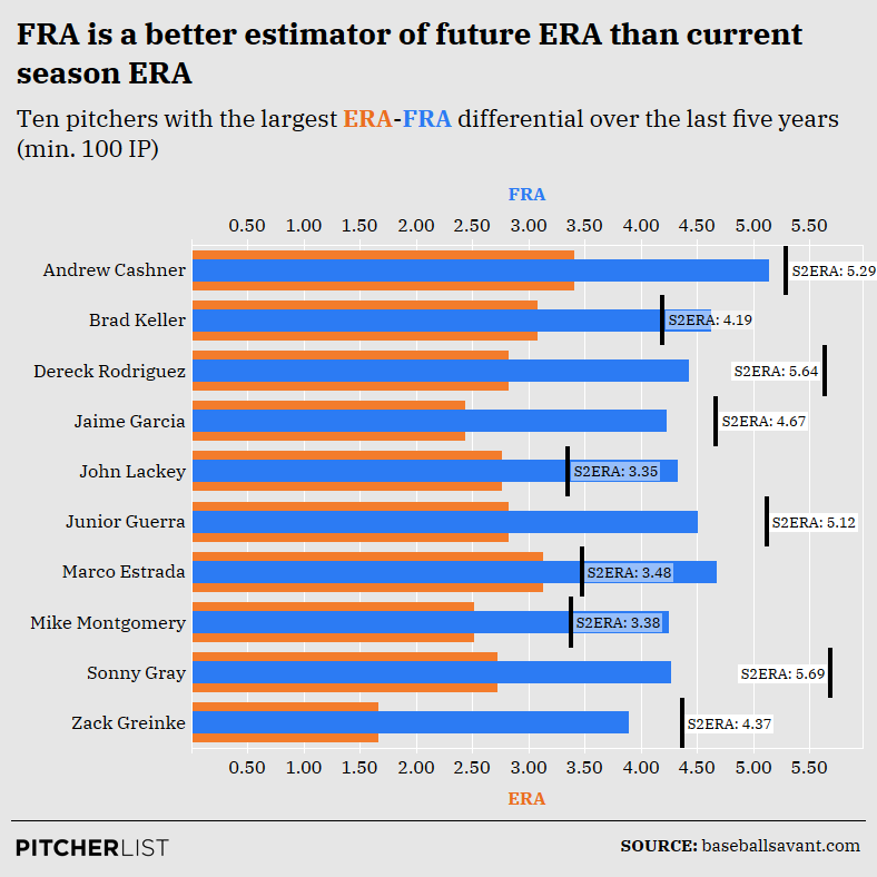
Data Visualization by Nick Kollauf (@Kollauf on Twitter)
With large FRA-ERA differentials, we would expect an increase in ERA the following year. And, indeed, there was such regression. In all ten cases, the pitcher’s ERA increased the following year. For seven of the ten pitchers, the FRA value was closer to the pitcher’s S2ERA than the ERA mark.
How much better off would you have been had you not paid up for Zack Greinke in 2016 based off his 1.66 ERA? I know he tanked at least one of my teams. Even if you never expected a sub-2.00 ERA to last and you had, instead, paid for a 3.00 ERA in 2016 drafts, his 4.37 ERA ultimately would have been detrimental at his draft-day cost. To that point, his 3.89 FRA was much closer to that mark and was premised upon his good (not great) 19.0 K-BB%–the most important component of FRA–as well as his suboptimal age (32).
Some of these pitchers likely weren’t draft targets in most leagues (e.g., Andrew Cashner, Mike Montgomery, Brad Keller). But, where it counted most, FRA was resoundingly more accurate than ERA. Of those remaining, you only would have been led astray with Marco Estrada, who nearly repeated his exceptionally low 2015 ERA of 3.13 in 2016. John Lackey, too, performed well the following year, though over half a run worse than in 2015. Even if you had missed out on them because of FRA, you would have correctly avoided Greinke, Jaime Garcia, Dereck Rodriguez, Sonny Gray, and Junior Guerra.
Now, consider 2019. Let’s peek at the ten biggest overperformers identified by FRA (min. 100 IP).
| Name | IP | Age | Age Score | K-BB% | aEV88.3 | ERA | FRA | ERA-FRA |
|---|---|---|---|---|---|---|---|---|
| Mike Soroka | 174.2 | 22 | 1 | 14.5 | 87 | 2.69 | 4.32 | -1.64 |
| Dakota Hudson | 174.2 | 25 | 7 | 6.6 | 88.3 | 3.36 | 4.86 | -1.50 |
| Hyun-Jin Ryu | 182.2 | 32 | 1 | 19.2 | 85.3 | 2.32 | 3.76 | -1.43 |
| Brett Anderson | 176 | 31 | 2 | 5.5 | 88.3 | 3.89 | 5.14 | -1.25 |
| Zach Davies | 159.2 | 26 | 9 | 7.6 | 87.4 | 3.56 | 4.60 | -1.04 |
| Jeff Samardzija | 181.1 | 34 | 4 | 12.3 | 88.3 | 3.53 | 4.53 | -1.01 |
| Dallas Keuchel | 112.2 | 31 | 2 | 10.7 | 88 | 3.77 | 4.70 | -0.93 |
| Sonny Gray | 175.1 | 30 | 5 | 19.4 | 87.1 | 2.88 | 3.80 | -0.92 |
| Zack Greinke | 208.2 | 36 | 3 | 19.4 | 86.8 | 2.94 | 3.84 | -0.90 |
| Marcus Stroman | 184.1 | 28 | 11 | 13 | 87.5 | 3.23 | 4.12 | -0.89 |
This time, I’ve included these pitchers’ FRA components so you can see exactly why they have worse FRAs than ERAs. Number one on this list is Mike Soroka. One observation I should make is that, of the 352 pitchers with back-to-back 100 IP from 2015-19, only two were 22 years-old, and their S2ERAs were poor. Thus, I stuck age 22 in the worst age score bucket (doing so also helped maintain a normal distribution of ages). With more data, I may move age 22 up, but for now, Soroka’s FRA may be artificially inflated because he’s one of the few 22-year-old pitchers in the league. Still, his K-BB% portends a much worse ERA than the 2.69 mark he earned, and his aEV was not so low as to counteract his Age Score and K-BB%.
On the one hand, Dakota Hudson, Brett Anderson, and Zach Davies each had extremely poor K-BB rates and aEVs. Their 4.50+ FRAs and large ERA-FRA disparities is, thus, unsurprising. On the other hand, Hyun-Jin Ryu, Greinke, and Gray’s inclusion on this list is perhaps surprising to some. Each had respectable FRAs right around 3.80. That is still useful for a fantasy team. The reason is that they all maintained good, albeit not earth-shattering, K-BB rates between 19.2-19.4%. Their aEVs also fell on the middle of the spectrum, with Ryu’s being quite low. However, they are all at least 30-years-old, earning low Age Scores. If you agree that earning the ERA of an ace without the K-BB% to match and doing so at, conceptually, a bad age to pitch, then you should expect regression for these pitchers.
That leaves Jeff Samardzija, Dallas Keuchel, and Marcus Stroman. One thing I noticed in the original FRA article was that the model seems to miss some pitchers who can outperform their ERAs with high ground ball rates. I did, in fact, test GB% as well as aLA and, had their been additional predictive power gleaned from either (no matter how minimal), the elastic net regression would have kept them.
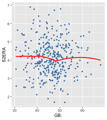
Yet, you can see it’s hard to discern a relationship between GB% and S2ERA–even at the extremes. On the high end of GB%, there are pitchers with both high and low S2ERAs. Nonetheless, it’s possible that, in some cases, a high GB% enables a pitcher to outperform his ERA based on some unexplained factors. Thus, of the ten names on this list of overperformers, seven are in the top-15 in GB% (min. 100 IP) according to FanGraphs. That includes Keuchel (no. 1) and Stroman (no. 6). Both had middling K-BB rates (10.7% and 13.0%, respectively) and relatively high aEVs, thereby earning significantly higher FRA marks than their ERAs. Separately, for his part, Samardzija is simply an older pitcher with an unimpressive K-BB rate who also gets hit quite hard, meaning you should expect regression.
You may be wondering why I’m focusing on overperformers instead of underperformers. The biggest underperformers largely had ERAs over 6.00 (e.g., Jordan Zimmerman, Drew Smyly, Jorge Lopez). For fantasy analysis, saying these largely nonrelevant pitchers will regress to their 4.50 FRAs piques my interest less than the other side of the coin. However, note also that Chris Sale and his 3.13 FRA would have made a list of top 10 2019 underperformers.
That raises an interesting issue, however, in that FRA’s variance is smaller than ERA’s. From 2015-19, although the FRA mean was 4.20 and the ERA mean was similarly 4.14 (again, min. 100 IP), the standard deviation for ERA was 0.92, whereas FRA’s was 0.48. In other words, the degree of spread of ERAs was much larger than of FRAs, as FRA regresses pitchers closer to the mean. Therefore, you simply don’t get many FRA values under 3.00 or over 5.00. I addressed this in my last article as follows:
FRA’s regression to the mean is deliberate and reasonable. It enables better ERA predictions because pitchers tend to run unremarkable K-BB rates. In short, some pitchers may experience good or bad luck in a given season, resulting in an ERA under 3.00 or over 5.00. However, unless their underlying skills are as bad as [Mike] Pelfrey’s (in which case they’re likely out of the league) or as good as Gerrit Cole’s (34% K-BB rate, [2.66] FRA in 2019), they generally will not repeat outlier ERAs, which is why FRA’s conservative predictions are more accurate than others.
Lastly, I’d like to make a few observations about pitchers with surprisingly low 2019 FRAs:
- Inspired by his impressive 22.9 K-BB% and peak age, FRA has assigned Brandon Woodruff the sixth-best FRA mark (3.20) among all 2019 pitchers with at least 100 IP.
- Similarly, Matthew Boyd has the 11th-best 2019 FRA (3.37), which was the result of his elite 23.9 K-BB% and high Age Score. A word of caution, however, that he also had a very high aEV.
- The same can be said for Robbie Ray, with a 3.48 FRA, 20.3 K-BB%, 86.9 aEV, and entering his age-29 season. You may be skeptical and think FRA will always miss something about Ray given he usually can’t pair a low ERA with his elite strikeout ability. I’d respond by noting that his FRA was 4.32 in 2015, 3.58 in 2016 (when he had an amazing 2.89 ERA and tanked the following year), and 3.90 in 2016. The model is more nuanced than simply assuming that Ray will have a low FRA because of his high K-BB%.
- Ryan Yarbrough wound up quite high on the FRA leaderboard as well–number 12, just behind Boyd–with a 3.38 FRA. While I think he could be better than his 4.14 ERA, I do not expect such a low ERA in 2020. Frankly, it’s a stretch to say he was the 12th-best pitcher to throw at least 100 innings last year. To that point, his 17.2 K-BB% was lower than the next 22 pitchers after him on the list, all the way through number 34, Caleb Smith. The reason his FRA was nevertheless so good is that he posted an exceptionally low aEV of 84.1 mph–the absolute lowest of 2019 pitchers with 100 IP–and he earned the highest age score because he was exactly 28-years-old in 2019. Yet, something doesn’t sit right with me about relying on the periphery variables to earn such a low FRA. Who knows if such an outlier aEV is even sustainable. In other words, Yarbrough’s FRA serves as a helpful warning against just looking at FRA without examining the model’s components for an individual pitcher.
- Kevin Gausman might still have something left in the tank, as evidenced by his 3.64 FRA–a full 2.09 runs below his atrocious ERA. Nonetheless, his FRA is likely inflated by an 18.2 K-BB% that was earned, in part, by bullpen work in 2019, as well as a peak Age Score. The exact same can be said for 28-year-old Matt Strahm, his time spent in the bullpen, and his resulting 3.66 FRA. Even though these are more reasonable FRA values than Yarbrough’s, and these pitchers had better K-BB rates, I am still skeptical they will post ERAs under 3.70.
- Trevor Bauer earned a 3.74 FRA, which is a far cry from his 4.48 ERA, due to a solid 18.8 K-BB% and peak Age Score. He gets hit hard and plays in notoriously hitter-friendly GABP, but is probably better than what he was last year, even if he’s not as good as his ridiculous 2018.
- Adrian Houser and Caleb Smith are similar pitchers who represent great late-round value in drafts this year. Considering they’re both entering their primes and they have similar, decent K-BB rates (17.3% for Houser, 16.7% for Smith), it’s no surprise they had relatively low FRAs (3.68 for Houser, 3.82 for Smith).
- Joe Musgrove and Dylan Bundy both had unexpectedly low FRAs: 3.98 and 4.04, respectively. They are the right age to forecast an optimally low S2ERA. Musgrove outperformed Bundy in terms of K-BB% (16.5% vs 14.8%), but got hit harder. They’ll make for interesting late-round flyers, among others.
And, on pitchers with surprisingly high FRA marks in 2019:
- Clayton Kershaw’s 3.81 FRA can be attributed to his relatively high aEV (87.1 mph) and extremely low age score. Remember that S2ERA peaks where pitchers were 31 & 32 the year prior, such as 31-year-old Kershaw. His skills were still excellent–21.0 K-BB%–so, if you believe that his inauspicious age is not actually prescient, then you shouldn’t buy his relatively high FRA. But, if you agree with FRA that, conceptually, being 31-years-old is a bad thing for a pitcher, then you should proceed with caution.
- Likewise, Patrick Corbin has a great K-BB rate of 20.1%, but he’s getting dangerously close to the worst part of the age curve, and he gets hit exceptionally hard. In fact, his aEV was so high (88.9 mph) that he’s one of the pitchers whose aEVs was changed to 88.3 mph for purposes of the model. Of course, if he actually performed to his 3.89 FRA next year, that would still be fine for a fantasy team, but it wouldn’t be worth paying his price in drafts.
- James Paxton had very similar results to Corbin and Kershaw. A 20.7 K-BB% (great!), though he was penalized due to an 88.3 mph aEV (changed from 88.6 mph) and being 31-years-old.
- The model suggests that Aaron Nola earned his 3.87 ERA given his 3.94 FRA. Nola’s 17.5 K-BB% is one of the worst discussed to this point, as is his 88.3 mph aEV (changed from 88.5 mph). Although he is still young, based on his other skills relevant here, I would not expect a bounceback.
- Mike Minor and Cole Hamels might be gassed. Minor had a 4.19 FRA and Hamels a 4.43 FRA. Minor’s at the absolute highest point of the age~S2ERA curve and Hamels is at the tail – not good places to be. Plus, they ran poor K-BB rates of 15.3% and 14.1%, respectively.
Conclusion
I’ll conclude briefly and similarly to the original FRA post. FRA is a step in the right direction, as it is more predictive of S2ERA than any of ERA, FIP, xFIP, SIERA, xERA, or DRA, and stickier, too. This time, it is battle tested, with even the worst test results outperforming the predictive capabilities of other ERA estimators. Again, you can find a list of all FRAs dating back to 2015 (min. 100 IP) here.
Although FRA is stickier and more predictive than other ERA estimators, bear in mind that it still only explained 24.5% of the variance in the S2ERA sample. Accordingly, there remains substantial unexplained variance in approximating future ERA. ERA is a fickle statistic subject to a substantial amount of randomness year-to-year that FRA will miss.
Featured Image by Rick Orengo (@OneFiddyOne on Twitter and Instagram)
Great stuff.
You don’t include kwERA in your comparison, but I see this as taking it to the next level. We’ve known since DIPS that K/BB% will explain a lot of a pitcher’s run prevention.
However, a few pitchers who still succeed despite a poor K/BB%. Their usual secret is inducing weak contact, which you are able to capture with aEV.
Thank you! Funny enough, kwERA was actually brought to my attention hours before the original FRA post ran, which required me to add a sentence acknowledging it.